CREATING AN ESRI SHAPEFILE WITH BATHYMETRY CONTOURS FROM POINT DATA USING QGIS
This article shows how to use QGIS operations to convert Excel bathymetry point data to depth contours. When bathymetry readings are provided from measurements at many points in a body of water, the goal is to create polygons around all points with depth classes, and remove land areas using clipping.
CSV Preparation
Data reduction
I was given an Excel file containing over 200,000 points of data:
| latitude | longitude | depth |
|---|---|---|
| 24.23035 | 23.5454 | 9.544293 |
| 24.23038 | 23.5456 | 9.326215 |
| 24.24042 | 23.5458 | 12.969445 |
| … | … | … |
This much data is too much for QGIS to handle. For a contour map, I also didn’t need that much detail. Data can be simplified by keeping (for example) only every 100th row, reducing it to 2,000 data points. In Excel, this can be done using the following formula:
=OFFSET(DepthSheet!$A$1,(ROW()-1)*10,0)Creating this formula in a new sheet, and copying it by dragging down 2,000 times produces a new worksheet with simplified data.
Adding depth categories
The contours we will be creating need discrete depth classes. In my Excel data, there are columns latitude, longitude and depth, where depths are anywhere between 0m and 35m, with up to 6 significant digits. For contour polygons, this level of detail is not desirable and depths should be expressed in classes (0-5m, 5-10m, etc.) To do this, Excel offers the MROUND function:
=MROUND(ABS(C2),5)This produces multiples of 5 (i.e. 0, 5, 10, 15, …) which will be the classes. We will place them in a new column called class, so that we get:
| latitude | longitude | depth | class |
|---|---|---|---|
| 24.23035 | 23.5454 | 9.544293 | 1 |
| 24.23038 | 23.5456 | 9.326215 | 1 |
| 24.24042 | 23.5458 | 12.969445 | 2 |
| … | … | … |
The resulting file (with the additional class column) can now be exported to CSV.
QGIS Manipulation
Reading CSV
QGIS can read point data from a CSV file using Layer -> Add Layer -> Add delimited text layer. Default options work.
Voronoi polygons
The input list of points must be converted to a set of polygons, all of which must have shared edges. One way to do this is to create Voronoi polygons. This creates a polygon around each point which edges equidistant to each neighbouring point.
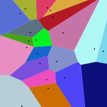
QGIS offers Voronoi diagram creation under Vector -> Geometry tools -> Voronoi polygons. The Voronoi polygons tool has an option to set a buffer region. This is the amount by which the resulting polygons will extend beyond the perimeter points. Setting it to 50% will help clipping later.
For 2,000 points this works well, while 20,000 points hangs QGIS. This appears to be a limitation of QGIS’s Python implementation of the Voronoi algorithm, since algorithms exist that can handle many more points and produce results in seconds - but using them would require leaving QGIS.
The Voronoi diagram algorithm will keep the latitude, longitude and depth fields. These can be removed in the QGIS Attribute Table. Only the class field need be kept.
Polygon dissolution
Polygons with the same depth class may be joined (dissolved). QGIS offers this under Vector -> Geoprocessing Tools -> Dissolve. The class field must be selected to dissolve on. Dissolve all must be unselected.
Clipping
The dissolved polygons must be clipped with the area originally occupied by the input points. This can be done using Vector -> Geometry Tools -> Delaunay Triangulation, followed by a Dissolve on all fields, which produces a single polygon.
Vector -> Geoprocessing Tools -> Clip will clip the dissolved Voronoi diagram with the clip area.
Clipping may cause the class field to become of string type. To change it back to integer, use Refactor fields in the QGIS toolbox. This will create a new layer.
Note that Delaunay triangulation creates a convex shape. For concave shapes, it is better to use the Concave hull algorithm found in the QGIS toolbox - though there is no true concave hull and this is merely an approximation.
Smoothing
The clipped result will be blocky, consisting of clearly visible Voronoi cells. This can be improved using the GRASS toolkit, with the v.generalize.smooth tool. Various methods are available, giving different results:
Boyle 
Chalken 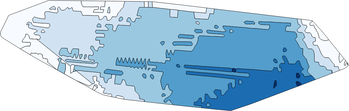
Distance weighting 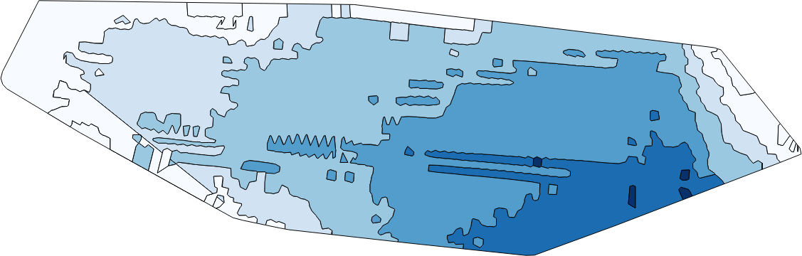
Hermite 
Sliding averaging 
Snakes 
The Snakes method appears to produce rounded polygons suitable for depth contours. The output shown is for default parameters.
Output
The resulting smoothed layer can now be saved as an ESRI shapefile.